We generated the freshwater hazard indicator data contained in the Data Portal based on a multi-model ensemble (MME) approach (Sect. 1). In parallel, methods for Providing and Utilizing eNsemble Information (PUNI) were co-developed jointly by global hydrological modelers, scientists investigating co-development methods and societal information needs, boundary organizations and stakeholders (Sect. 2).
1. Impact modelling
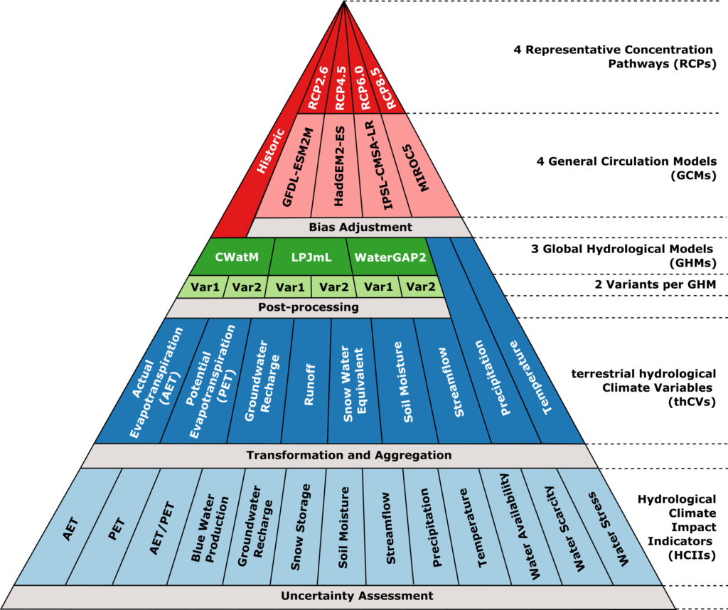
Future climate conditions can be estimated by driving general circulation models (GCMs) based on Representative Concentration Pathways (RCPs). The future climate scenarios obtained in this way can be used as input in global hydrological models (GHMs) to derive future freshwater-related hazards of climate change. It is state-of-the-art to consider multiple RCP-GCM-GHM combinations rather than a single one in climate impact assessments: this is known as the multi-model ensemble approach.
The CO-MICC MME is based on a selection of multiple RCPs, GCMs and GHMs (Fig. 1) that builds on the framework provided by the Inter-Sectoral Impact Model Intercomparison Project (ISIMIP). Bias-corrected GCM-driven simulations of multiple GHMs were carried out to produce MME data of terrestrial hydrological climate variables (thCVs) at global scale.The MME data of thCVswere aggregated at different scales and used to derive MME data of hydrological climate impact indicators (HCIIs), which are provided in the Data Portal.
1.1 Climate projections
We used the climate input data of the ISIMIP2b simulation round to force the global hydrological models. This was done to enable comparability to ISIMIP2b multi-model ensemble runs in the analysis. Below, we briefly describe how these climate input data were generated.
Historical (1861-2005) and future climate conditions were simulated by multiple GCMs in the framework of the Coupled Model Intercomparison Project Phase 5 (CMIP5). The output data from the following four GCMs was used for ISIMIP2b:
- IPSL-CM5A-LR
- GFDL-ESM2M
- MIROC5
- HadGEM2-ES
To account for future human-induced greenhouse gas (GHG) emission scenarios, the GCMs were forced by the RCPs adopted by the Intergovernmental Panel on Climate Change for its Fifth Assessment Report (AR5) in 2014:
- RCP2.6 (lowest GHG emission scenario)
- RCP4.5
- RCP6.0
- RCP8.5 (highest GHG emission scenario)
Each of these pathways is based on a set of assumptions about economic activity, energy sources, population growth and other socio-economic factors, and contains emission estimates up to the year 2100. The aim of including all four RCPs is to increase the number of ensemble members and, in this way, to better represent the uncertainty of future climate projections. For more detailed information concerning the RCPs, please consult The Beginner’s Guide to Representative Concentration Pathways by Graham Wayne.
In the framework of ISIMIP2b, the original output data from the GCMs was bias corrected based on the EWEMBI (EartH2Observe, WFDEI and ERA-Interim data Merged and Bias-corrected for ISIMIP) observational dataset, which covers the entire globe at 0.5° horizontal spatial resolution and daily temporal resolution from 1979 to 2013. For more detailed information concerning the bias correction, please consult the ISIMIP2b Bias Correction Fact Sheet. The resulting ISIMIP2b climate input data set has a daily temporal resolution and a 0.5° horizontal spatial resolution. In the context of CO-MICC, future GCM runs were carried out over 30-year time periods centered from 2020 to 2085 in 5-year time steps.
1.2 Hydrological projections
1.2.1 Global hydrological models
Four well-established GHMs participated in CO-MICC:
- The Community Water Model (CWatM) version 1.04, developed at the International Institute for Applied Systems Analysis (IIASA), in Austria
- The Lund-Potsdam-Jena managed Land (LPJmL) model version 5.0, developed at the Potsdam Institute for Climate Impact Research (PIK), in Germany
- The ORganising Carbon and Hydrology In Dynamic EcosystEms (ORCHIDEE) land surface model version ORCHIDEE_gmd-2018-57, developed at the Dynamic Meteorology Laboratory (LMD) of the Pierre Simon Laplace Institute (IPSL), in France
- The Water Global Assessment and Prognosis model version 2.2d (WaterGAP2.2d), developed at the Institute of Physical Geography (IPG) of the Goethe University Frankfurt (GUF), in Germany
These models simulate the terrestrial water cycle with its water flows, water storage compartments and human water use sectors (except ORCHIDEE, which neglects human impacts on water flows and storages), on the global scale. They can assess past and future impacts of climate change on freshwater systems. Despite their common applications, these GHMs were developed within different modelling frameworks and have distinct foci, leading to fundamental differences in model structure and model parameterization.
LPJmL and ORCHIDEE are used by both the global hydrological and the global vegetation communities, as not only can they be classified as GHMs, but they also fall into the category of Dynamic Global Vegetation Model (DGVM). Unlike the other GHMs, LPJmL and ORCHIDEE have an advanced representation of vegetation dynamics by means of a dynamic vegetation module, which simulates the evolution of vegetation with climate. In addition to vegetation composition and distribution, they also simulate the terrestrial carbon and water cycles. LPJmL considers both natural and agricultural ecosystems, whereas ORCHIDEE is restricted to natural ecosystems.
CWatM and WaterGAP2.2d are global water resources and water use models. They are comparable in terms of structure, parameterization and the main motivations behind their development. They were designed with the purpose of quantitatively assessing water availability, water demand and environmental needs. A major focus in these models is the representation of human water use in multiple sectors (irrigation, domestic, industrial and livestock) as water abstractions from surface water and groundwater, and reservoir operations. They consider multiple land cover classes, but have no dynamic vegetation module.
All four models were part of the model evaluation phase of the project. However, only three out of four, namely CWatM, LPJmL and WaterGAP2.2d, were used to generate project-specific MMEs of future impacts of climate change on freshwater systems. These GHMs were run over a reference period (1981-2010) and over 30-year time periods centered from 2020 to 2085 in 5-year time steps. The inclusion of ORCHIDEE as part of the CO-MICC impact models is expected to happen at a later stage.
CWatM, LPJmL and WaterGAP2.2d run at daily temporal resolution over a global grid divided into 0.5° by 0.5° cells (55 km by 55 km at the equator and ~3000 km2 grid cell). The grid covers the global continental area except for Antarctica. Outputs are generated as daily, monthly or annual spatially explicit time series.
To increase the number of ensemble members and thus better account for uncertainty in the model projections, each GHM was run according to two modelling schemes differing from one another in the way potential evapotranspiration (PET) is calculated. PET is one of the most sensitive (and thus uncertain) variables in the water balance equation of GHMs. As it is the sum of evaporation from the soil and transpiration from the vegetation, this variable depends on vegetation characteristics and processes. Among other factors, the latter are sensitive to changing atmospheric CO2 concentrations. DGVMs such as LPJmL are able to explicitly simulate the active response of vegetation to this forcing through the inclusion of a dynamic vegetation module. CWatM and WaterGAP2.2d, on the other hand, do not include a dynamic vegetation module and are thus unable to explicitly simulate the active response of vegetation. Nevertheless, these models can mimic this response by adapting their PET equation. In WaterGAP2.2d, the default is to calculate PET according to the Priestley-Taylor approach: hereafter, we refer to this as the “PET-PT scheme”. The PET-PT scheme does not account for PET changes due to the effects of the active vegetation response to changing atmospheric CO2 concentrations. As an alternative to the default, WaterGAP2.2d was also run according to a non-standard scheme based on Milly and Dunne (2016) which accounts for these PET changes: hereafter, we refer to this as the “PET-MD scheme”. These two modelling schemes made it possible to include the impacts of a non-climatic driver, namely the rising CO2 concentrations, on freshwater systems in the MMEs.
Moreover, the models were run under two different modes:
- the anthropogenic mode (standard mode), which includes both climate- and human-induced impacts, and
- the naturalized mode, which neglects human water abstractions as well as the construction and operation of artificial reservoirs.
Most of the hazard indicators in the data portal were generated from the outputs of the anthropogenic model runs. On the other hand, naturalized runs were required to generate the indicators related to blue water production and naturalized streamflow (see Freshwater Hazard Indicators).
1.2.2 Model evaluation
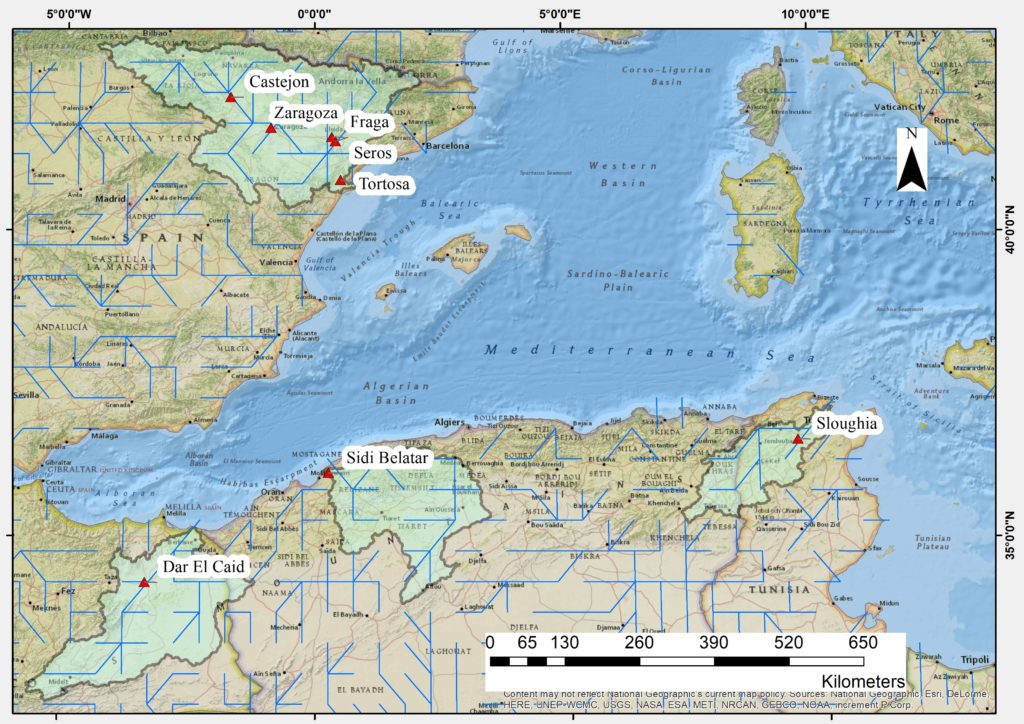
The performance of the GHMs was evaluated prior to their usage to simulate future freshwater availability conditions. As is common practice in the hydrological modelling community, the performance of the models was assessed by testing their capacity to reproduce past conditions. The assumption behind is that, if the models are capable to reproduce past conditions with an acceptable degree of accuracy, then they can be trusted to simulate future conditions with a similar degree of accuracy. Concretely, model estimates of streamflow were compared to in situ observations at gauging stations in the CO-MICC focus regions (Fig. 2 and Table 1) over historical time periods. Four Mediterranean basins were selected as focus regions. The Ebro basin is located in Eastern Spain. The other three basins, namely the Moulouya, Chelif and Wadi Majardah (also known as Medjerda) basins, are distributed between Morocco, Algeria and Tunisia (MAT region).
The observations were obtained from the data portal of the Global Runoff Data Centre (GRDC). The models were forced with the daily-resolution observed global climate data set from the Global Soil Wetness Project Phase 3 (GSWP3), based onthe reanalysis data set 20CR and using the bias targets GPCC, GPCP, CPC-Unified, CRU and SRB. The evaluation period considered was 1914-1980 because it is the earliest time period with sufficient coverage of observations for all stations. The earliest possible period was chosen to reduce the water-related anthropogenic activities that are not considered in the GHMs, assuming that the hydrology of these basins is less impacted by humans during that period.
Table 1: Attributes of gauging stations used for model evaluation.| Station name | GRDC station code | Longitude | Latitude | River name | Drainage area (km2) | Elevation (m.a.s.l.) |
|---|---|---|---|---|---|---|
| Fraga | 6226650 | 0.35 | 41.52 | Cinca | 9612 | 100.0 |
| Seros | 6226600 | 0.42 | 41.45 | Segre | 12782 | 85.0 |
| Castejon | 6226300 | -1.69 | 42.18 | Ebro | 25194 | 265.0 |
| Tortosa | 6226800 | 0.52 | 40.81 | Ebro | 84230 | 25.0 |
| Zaragoza | 6226400 | -0.88 | 41.66 | Ebro | 40434 | 189.0 |
| Dar El Caid | 1308600 | -3.32 | 34.24 | Moulouya | 24422 | 325.0 |
| Sidi Belatar | 1104150 | 0.27 | 36.02 | Chelif | 43750 | 2.0 |
| Sloughia | 1201500 | 9.52 | 36.58 | Majardah | 20895 | 67.0 |
The first stage of model evaluation consisted in evaluating how well the models can reproduce the mean seasonal variability and the annual variability of the observed streamflow.
In general, the models showed a poor performance in terms of mean seasonal streamflow variability. The poor fit between observations and model estimates could be due to several factors. For instance, it could stem from the climate input data used by the models, from how the models simulate runoff generation and/or from how the models simulate water use and dam operation. Another factor could be the presence of water transfers, which are not considered by the models. GHMs are not well enough informed to simulate the local water-related anthropogenic activities. Nevertheless, the focus of the CO-MICC project is not on simulating the local anthropogenic activities but on translating global climate signals into hydrological responses.
Unlike for mean seasonal streamflow variability, the models showed a good performance in terms of annual variability. Based on the Kling-Gupta efficiency (KGE) metric, the models perform better regarding the correlation and variability than the bias (Table 2). Furthermore, the comparison between the annual streamflow simulated in anthropogenic mode to the one obtained in naturalized mode showed smaller differences between the two modes than for the mean seasonal streamflow. From this, it was inferred that the annual streamflow variability is likely less influenced by human impacts (dams, water use) and more influenced by climate variability than the mean seasonal variability. Given that the focus is on translating global climate signals into hydrological responses, this implies that the annual streamflow variability is a more suitable indicator for evaluating the reliability of the outputs generated by the GHMs.
Table 2: Goodness of fit between observed and modelled annual streamflow in eight gauging stations based on the Kling-Gupta Efficiency (KGE). The KGE consists of three individual components, namely the correlation (r), bias (beta) and variability (gamma). Values of the KGE, r, beta and gamma closer to 1 suggest a better fit.| Model | Parameter | Fraga | Seros | Castejon | Tortosa | Zaragoza | Dar El Caid | Sidi Belatar | Sloughia |
|---|---|---|---|---|---|---|---|---|---|
| WaterGAP2 | KGE | 0,76 | 0,848 | 0,619 | 0,5 | 0,238 | -0,844 | -5,52 | -4,158 |
| r | 0,924 | 0,892 | 0,937 | 0,712 | 0,841 | 0,902 | 0,965 | 0,788 | |
| Beta | 0,979 | 0,909 | 1,364 | 0,865 | 1,728 | 1,759 | 4,56 | 5,289 | |
| Gamma | 0,774 | 0,945 | 1,095 | 0,615 | 1,161 | 2,678 | 6,462 | 3,857 | |
| LPJmL | KGE | 0,611 | 0,73 | 0,668 | 0,45 | 0,392 | -5,827 | -10,476 | -9,973 |
| r | 0,916 | 0,882 | 0,882 | 0,614 | 0,812 | 0,939 | 0,966 | 0,96 | |
| Beta | 0,732 | 1,238 | 1,302 | 1,391 | 1,568 | 6,414 | 8,64 | 9,647 | |
| Gamma | 0,73 | 1,047 | 1,073 | 1,026 | 1,113 | 5,159 | 9,563 | 7,756 | |
| CWatM | KGE | 0,273 | 0,522 | 0,783 | 0,573 | 0,414 | -2,518 | -6,347 | -6,214 |
| r | 0,858 | 0,743 | 0,932 | 0,659 | 0,843 | 0,929 | 0,978 | 0,955 | |
| Beta | 0,559 | 0,892 | 1,197 | 1,2 | 1,561 | 3,675 | 6,296 | 6,86 | |
| Gamma | 0,439 | 0,611 | 1,06 | 0,838 | 1,069 | 3,283 | 6,093 | 5,206 | |
| ORCHIDEE | KGE | 0,671 | 0,558 | 0,687 | 0,285 | 0,705 | -1,665 | -2,757 | -1,889 |
| r | 0,849 | 0,731 | 0,886 | 0,502 | 0,776 | 0,916 | 0,999 | 0,97 | |
| Beta | 1,218 | 1,332 | 0,773 | 0,808 | 0,967 | 2,992 | 3,911 | 2,929 | |
| Gamma | 0,804 | 0,885 | 0,818 | 0,524 | 0,81 | 2,769 | 3,375 | 3,15 |
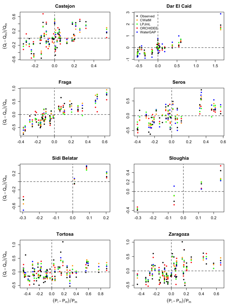
With that in mind, the second stage of model evaluation consisted in looking into two additional indicators, namely the interannual variability of annual streamflow (Fig. 3) and the sensitivity of annual streamflow to precipitation variability (Fig. 4).
In general, the GHMs agree reasonably well with the interannual variability of the observed annual streamflow. Moreover, the GHM-based annual streamflow response to precipitation variability is close to the observed annual streamflow response. The conclusion drawn from these results was that the GHMs are capable of translating the climate signal into a hydrological response, with some uncertainty.

2. Stakeholder engagement
2.1 Participating stakeholders
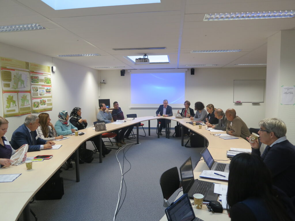
Throughout the project lifecycle, numerous stakeholders with different backgrounds, needs and expectations were interviewed and actively invited to take part in workshops organized by the project partners. These workshops consisted in participatory processes during which the scientists (climate knowledge and information providers) and the stakeholders (climate knowledge and information users) co-designed PUNI (Providing and Utilizing eNsemble Information) methods. This was achieved by iteratively testing alternative ways of presenting and utilizing MME data in support of exemplary climate change risk assessments. The idea behind the implementation of co-design processes in the portal development cycle was to create a demand-driven climate service, with easy-to-understand and easy-to-use climate information.
Two main groups of stakeholders can be distinguished: one composed of stakeholders from the public sector in the CO-MICC focus regions, and the other of stakeholders from globally operating companies.
The participating stakeholders from the CO-MICC focus regions were basically experts and decision-makers from meteorological services, research institutions, basin agencies, ministries, and intergovernmental institutions. The motivation of this type of stakeholder to use climate services is based on the potential of such tools to support informed planning and decision-making in the context of climate change. The ultimate goal is to ensure a sustainable water management at the basin and country levels for all sectors in the future.
Concerning globally operating companies, their increasing interest in climate services has different motivations. On the one hand, these companies are integrating climate change risk assessments in relation to their production sites and key supply chains as part of their business strategy. For instance, such assessments can help them identify sites that are projected to suffer from water stress issues in the foreseeable future, allowing them to adapt their plans accordingly.
On the other hand, companies in general are aiming to become more sustainable. A key step in their journey to become greener is the reduction of their water footprint. In this context, the usage of climate services which include water-related indicators can help them assess whether their planned future activities might exacerbate the projected water stress in a certain region or country.
The following sections present the main results of the interviews that were carried out in the three focus catchments of the MAT region (Fig. 2) to investigate the risk perception (Sect. 2.2) and information needs (Sect. 2.3) of stakeholders for water management in the face of climate change.
2.2. Risk perception
2.2.1 Perception of the climate
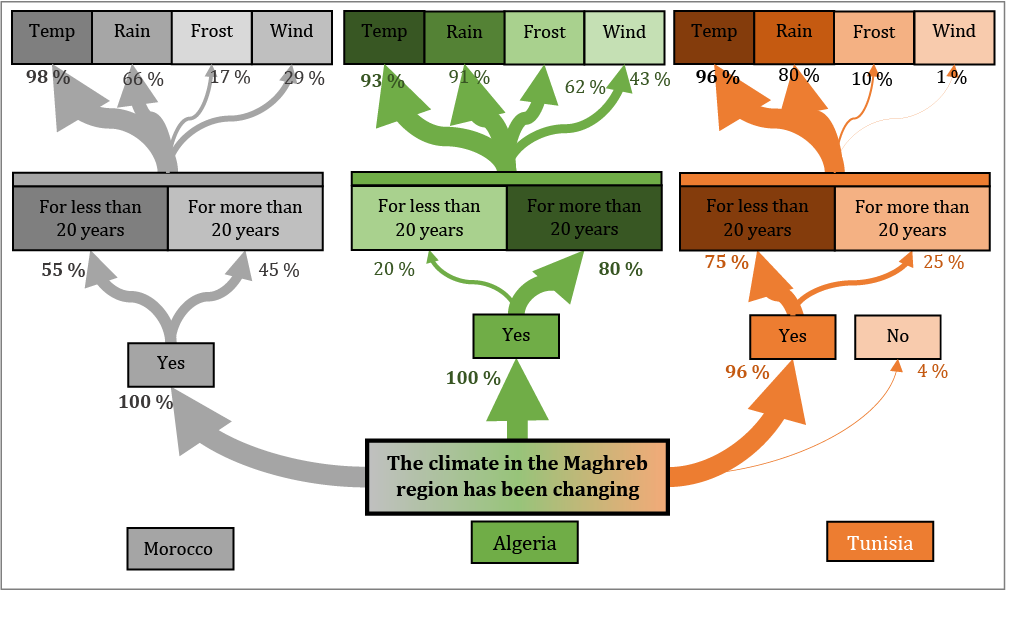
The majority of the surveys shows that the climate has been changing for about two decades (Fig. 6). This change is mostly perceived through several indicators: temperature increase, decrease of precipitation and wind effects. This is especially true of the catchment in Algeria, located at an altitude of more than 1000 m, with cold and frost posing a certain risk.
2.2.2 Perception of climate change
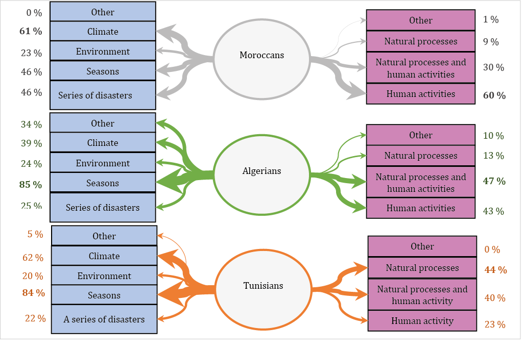
The surveys show a rate of climate change perception of more than 90 %. It is either of natural or anthropogenic origin or a combination of both. This change is perceived in the disruption of the seasons, the climate conditions, natural disasters (drought and floods) and the environment (Fig. 7).
2.2.3 Perception of risk and vulnerability
The effects of climate change are perceived through environmental problems concerning water resources: lack of water and drought, heavy rainstorms, floods, soil degradation and erosion.
These environmental problems had adverse effects on activities as well as on tangible and intangible assets. The resulting damage concerns ruined agricultural land or livestock losses, the destruction of infrastructure and buildings and human casualties (Fig. 8).

2.2.4 Impacts on the perception of users towards climate change
The whole bundle of these disturbances impacts on all activities. When they think of climate change, the users feel sad, angry and anxious or scared (Fig. 9).

2.3 Information needs
First and foremost, the water users would like to obtain precipitation data (+ 90 %), especially concerning seasonal and autumnal precipitations. The users also require forecast data on temperatures, particularly relating to winter and spring temperatures. Indeed, there is a major demand for information on frost, snow and wind data (the latter to a lesser degree) for high-altitude sites (Fig. 10). In the three countries (Morocco, Algeria, Tunisia), the demand for hydrological data primarily concerns river discharge and groundwater levels (Fig. 10).

