The CO-MICC multi-model ensemble (MME) is based on a selection of multiple Representative Concentration Pathways (RCPs), General Circulation Models (GCMs), Global Hydrological Models (GHMs) and variants of the latter (hereafter referred to as “GHM variants”). This selection comprises 4 RCPs, 4 GCMs, 3 GHMs and 2 GHM variants. Each ensemble member consists of a combination of 1 RCP, 1 GCM, 1 GHM and 1 GHM variant. There are 96 ensemble members in total (4 RCPs x 4 GCMs x 3 GHMs x 2 GHM variants).
Each ensemble member was run to compute a series of climate and hydrological variables (see Table 1). These variables are climate-dependent and thus relevant when assessing climate change impacts. They describe the state and changes of the hydrosphere on land. Different variables describe different freshwater compartments (e.g., soil, groundwater, snow).
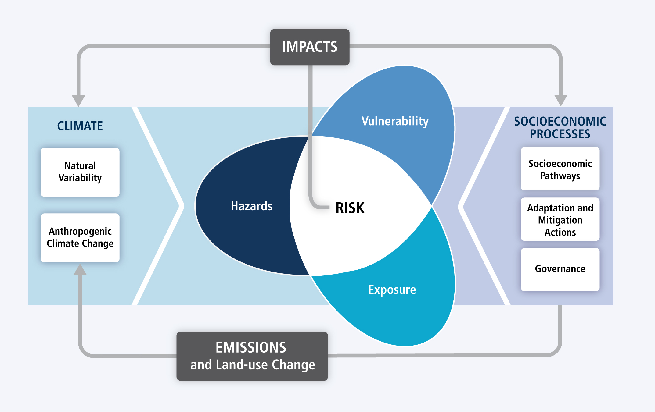
The Data Portal gives access to MME data of hydrological climate impact indicators (HCIIs). The risk of climate-related impacts results from the interaction of climate-related physical hazards with the vulnerability and exposure of human and natural systems (Figure 1). In other words, the risk of a climate-related impact is the probability of an event or a trend, multiplied by damage. The indicators considered here are specifically dedicated to quantifying the probability of climate-related physical hazards that have an effect on freshwater resources. In the following, we refer to them as hazard indicators.

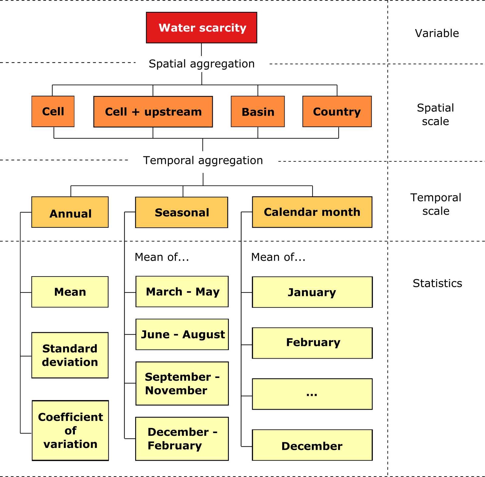
The calculation of hazard indicators based on the variables computed by the MME is done on-the-fly in the Data Portal. Multiple indicators can be derived from each variable. To derive a specific indicator, first, the variable in question is spatially and temporally aggregated and, secondly, a statistic based on the aggregated variable is calculated (Figure 2).

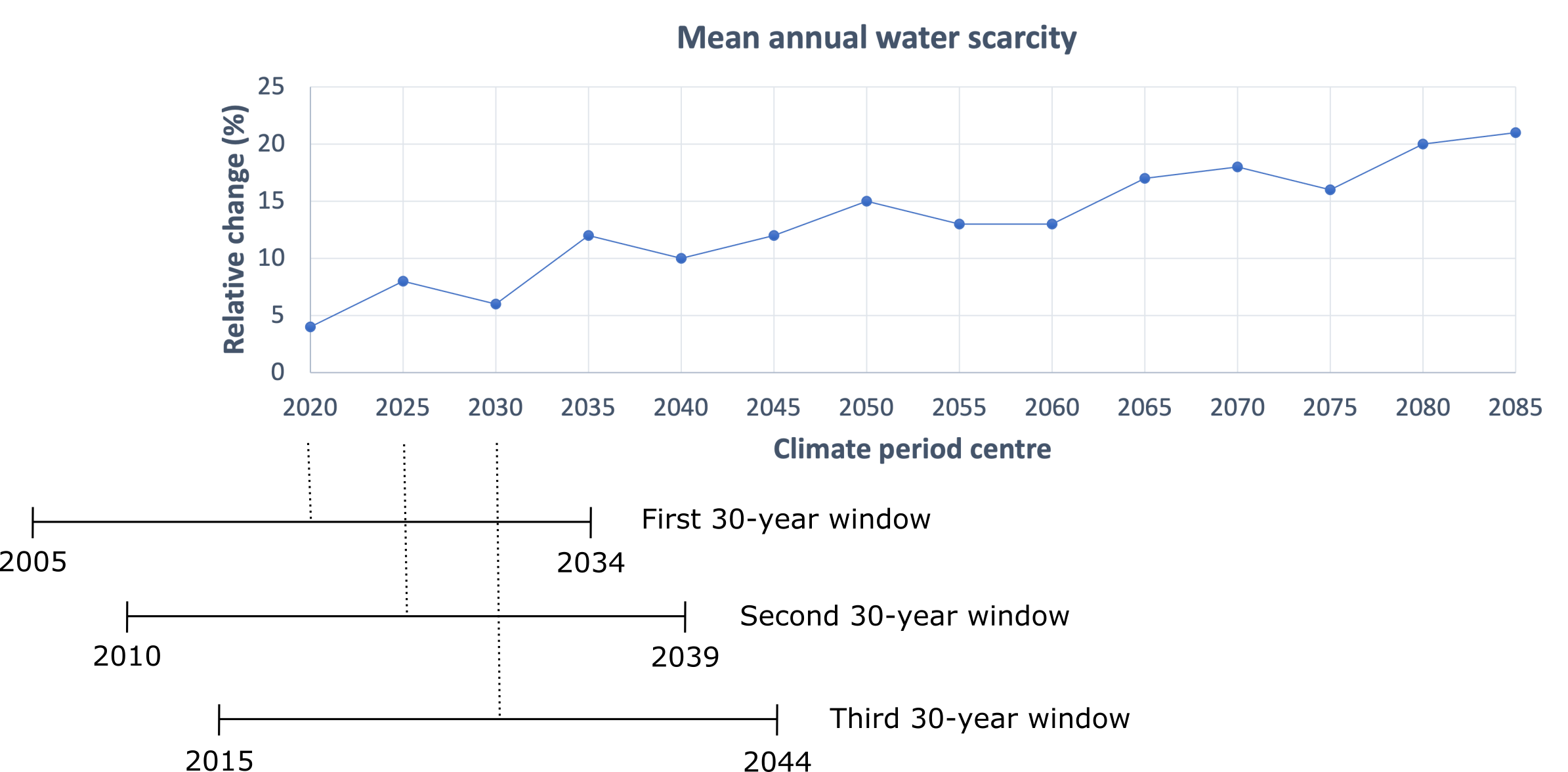
The values computed for a certain indicator correspond to either absolute or relative changes as compared to a reference value. This reference value is equal to the MME median value over the reference period 1981-2010. The projected absolute/relatives changes show how the indicator in question is expected to vary in the future according to different scenarios of climate change. By combining the simulated relative/absolute changes with the reference value, it is possible to obtain a rough estimate of the indicator in future time periods. Changes are averaged over future time periods of 30 years each. Fourteen future time periods are included in the Data Portal in total. In the time series chart that can be visualized in the latter, each time period is defined by its centre year (Figure 3). For example, the year 2030 actually refers to the period 2015-2044. The future periods are defined by a 30-year rolling window that shifts forward at a 5-year time step, resulting in overlapping periods (Figure 3).

In general, relative changes can be computed more reliably by the models than absolute changes. Relative changes should thus be favoured over absolute ones for climate change risk assessments. Only if relative changes are not available (e.g., in the case of water scarcity and water stress indicators), absolute changes should be considered. Relative changes are not provided in a certain grid cell if the MME reference value in that cell is equal to zero or smaller than a pre-defined threshold. Pre-defined thresholds were implemented to avoid very small reference values, which can lead to unreasonably large relative changes.
Table 1: Hazard indicators available in the CO-MICC Data Portal. These indicators correspond to multiple climate and hydrological variables computed by general circulation models and global hydrological models, respectively, over 30-year periods. They are provided at either annual scale, seasonal scale or for each calendar month.| Variable | Time scale | Statistic | Unit |
|---|---|---|---|
| Blue water production (BWP) | Annual | Mean | mm/year |
| Annual high: Q101 | mm/year | ||
| Annual low (1 in 10 years): Q901 | mm/year | ||
| Annual low (1 in 5 years): Q801 |
mm/year | ||
| Year-to-year variability: standard deviation | mm/year | ||
| Year-to-year variability: coefficient of variation | no unit | ||
| Streamflow (Q) | Annual | Mean | m³/s |
| Annual high: Q101 | m³/s | ||
| Annual low (1 in 10 years): Q901 | m³/s | ||
| Annual low (1 in 5 years): Q801 | m³/s | ||
| Monthly high: Q101 | m³/s | ||
| Monthly low: Q901 | m³/s | ||
| Year-to-year variability: standard deviation | m³/s | ||
| Year-to-year variability: coefficient of variation | no unit | ||
| Calendar month with highest mean monthly flow | month | ||
| Calendar month with lowest mean monthly flow | month | ||
| Seasonal | Mean of
|
m³/s | |
| Calendar month | Mean of
|
m³/s | |
| Naturalized streamflow (Qnat) | Annual | Mean | m³/s |
| Annual high: Q101 |
m³/s | ||
| Annual low (1 in 10 years): Q901 |
m³/s | ||
| Annual low (1 in 5 years): Q801 |
m³/s | ||
| Monthly high: Q101 |
m³/s | ||
| Monthly low: Q901 |
m³/s | ||
| Year-to-year variability: standard deviation |
m³/s | ||
| Year-to-year variability: coefficient of variation |
no unit | ||
| Calendar month with highest mean monthly flow |
month | ||
| Calendar month with lowest mean monthly flow | month | ||
| Seasonal | Mean of
|
m³/s | |
| Calendar month | Mean of
|
m³/s | |
| Potential evapotranspiration (PET) | Annual | Mean | mm/year |
| Year-to-year variability: standard deviation | mm/year | ||
| Year-to-year variability: coefficient of variation | no unit | ||
| PET/Precipitation | no unit | ||
| Seasonal | Mean of
|
mm/month | |
| Calendar month | Mean of
|
mm/month | |
| Actual evapotranspiration (AET) | Annual | Mean | mm/year |
| Year-to-year variability: standard deviation | mm/year | ||
| Year-to-year variability: coefficient of variation | no unit | ||
| AET/Precipitation | no unit | ||
| Seasonal | Mean of
|
mm/month | |
| Calendar month | Mean of
|
mm/month | |
| Groundwater recharge (GWR) | Annual | Mean | mm/year |
| Soil moisture (Ssoil) | Annual | Mean | no unit |
| Seasonal | Mean of
|
no unit | |
| Calendar month | Mean of
|
no unit | |
| Snow storage (Ssnow) | Annual | Mean | mm |
| Number of months with snow | month | ||
| Seasonal | Mean of
|
mm | |
| Calendar month | Mean of
|
mm | |
| Net irrigation requirement (NIR) | Annual | Mean | |
| Annual high: NIR102 | |||
| Annual Low: NIR903 | mm/year | ||
| Year-to-year variability: standard deviation | mm/year | ||
| Year-to-year variability: coefficient of variation | no unit | ||
| Temperature (T) | Annual | Mean | °C |
| Seasonal | Mean of
|
°C | |
| Calendar month | Mean of
|
°C | |
| Precipitation (P) | Annual | Mean | mm/year |
| Year-to-year variability: standard deviation | mm/year | ||
| Year-to-year variability: coefficient of variation | no unit | ||
| Calendar month with highest mean monthly precipitation | month | ||
| Calendar month with lowest mean monthly precipitation | month | ||
| R95T4 | no unit | ||
| Seasonal | Mean of
|
mm/month | |
| Calendar month | Mean of
|
mm/month | |
| Water scarcity (WSc) | Annual | Mean | no unit |
| Year-to-year variability: standard deviation | no unit | ||
| Year-to-year variability: coefficient of variation | no unit | ||
| Seasonal | Mean of
|
no unit | |
| Calendar month | Mean of
|
no unit | |
| Water stress (WSt) | Annual | Mean | no unit |
| Year-to-year variability: standard deviation | no unit | ||
| Year-to-year variability: coefficient of variation | no unit | ||
| Seasonal | Mean of
|
no unit | |
| Calendar month | Mean of
|
no unit | |
| Water availability (WA) | Annual | Mean | m³/year |
| Year-to-year variability: standard deviation | m³/year | ||
| Year-to-year variability: coefficient of variation | no unit | ||
| Seasonal | Mean of
|
m³/month | |
| Calendar month | Mean of
|
m³/month |
1 Q10, Q80, Q90: 10th percentile, 80th percentile, 90th percentile.
2 NIR10: annual net irrigation requirement that is exceeded in only 1 out of 10 years (i.e. net irrigation requirement in a dry year).
3 NIR90: annual net irrigation requirement that is exceeded in 9 out of 10 years (i.e. net irrigation requirement in a wet year).
4 R95T: fraction of annual total precipitation due to events exceeding the 1981-2010 period’s 95th percentile (i.e. fraction of annual total precipitation that occurred via extreme events).